1 Introduction
In most scientific disciplines one measures quantities that are affected by stochastic processes. Some examples are noise affecting electric signals, the different response by peoples to drugs due to differences at molecular level,…
In this document we introduce some fundamental results from probability theory and statistics that establish a relationship between measured quantities and the underlying stochastic processes. They thus allow to estimate the desired quantity and allow to give an indication of the error from the true value. By the latter we mean the value of the quantity if the stochastic process were not present.
We assume some knowledge about probability theory, but we start with a concise summary of the concepts that are needed. Throughout the document we’ll use a running example to illustrate the results.
2 Probability Refresher
A probability space is a triplet \((\Omega, \ensuremath{{\mathcal{F}}}, P)\). \(\Omega\) is the set of all possible outcomes of the experiment and is called sample space. An element \(\omega\) of \(\Omega\) is an elementary outcome and is called a sample point (or simply sample). Questions about the experiment are represented by subsets \(A\) of \(\Omega\) and called events. \(\ensuremath{{\mathcal{F}}} \subseteq \ensuremath{{\mathcal{P}}}(\Omega)\)1 is the collections of all possible events and technically must form a \(\sigma\)-algebra [1]. The function \[\begin{equation} \label{eq:P-def} P : \ensuremath{{\mathcal{F}}} \rightarrow [0, 1] \end{equation}\] gives the probability that an event occurs, i.e., \(P(A)\) is the probability of the occurrence of event \(A\in\ensuremath{{\mathcal{F}}}\).
Given a probability space \((\Omega, \ensuremath{{\mathcal{F}}}, P)\), a random variable is a function \[\begin{equation} \label{eq:random-var-def} X : \Omega \rightarrow \ensuremath{{\mathbb{R}}} \end{equation}\] such that for all \(a\in\ensuremath{{\mathbb{R}}}\) \[\{X \le a\} \ensuremath{:=} \{\omega\in \Omega\, |\, X(\omega) \le a\} \in \ensuremath{{\mathcal{F}}}\,.\] The cumulative distribution function (CDF) of \(X\) is the function \[\begin{equation} \label{eq:cdf-def} F_X(a)\ensuremath{:=}P(\{X \le a\})\,. \end{equation}\] If there exists a non-negative function \(p_X : \ensuremath{{\mathbb{R}}}\rightarrow \ensuremath{{\mathbb{R}}}\) such that \[\begin{equation} \label{eq:pdf-def} \int_{-\infty}^a p_X(x) \mathrm{d}x\ = F_X(a)\,, \end{equation}\] then it is called the probability density function (PDF) of \(X\). If the PDF of \(X\) exists and \(\int_{-\infty}^\infty \abs{x} p_X(x) \mathrm{d}x < \infty\) one defines the expected value of \(X\) by \[\begin{equation} \label{eq:expected-value-def} \operatorname{E}[X] \ensuremath{:=}\mu_X \ensuremath{:=}\int_{-\infty}^\infty x\, p_X(x) \mathrm{d}x\,. \end{equation}\] Similarly, if \(\int_{-\infty}^\infty x^2\, p_X(x) \mathrm{d}x < \infty\) one defines the variance of \(X\) by \[\begin{equation} \label{eq:variance-def} \operatorname{Var}(X) \ensuremath{:=} \int_{-\infty}^\infty (x - \mu_X)^2\,p_X(x) \mathrm{d}x\,. \end{equation}\] The positive square root \(\sqrt{\operatorname{Var}(X)}\) is called the standard deviation of \(X\) and denoted by \(\sigma_X\).
Given a random variable \(X\) and a function \(g:\ensuremath{{\mathbb{R}}}\rightarrow \ensuremath{{\mathbb{R}}}\), we can construct a new random variable \(Y=g(X)\). If \(\int_{-\infty}^\infty \abs{g(x)}\,p_X(x)\mathrm{d}x < \infty\), the expected value of \(Y\) is given by \[\operatorname{E}[Y] = \operatorname{E}[g(X)] = \int_{-\infty}^\infty g(x)\,p_X(x) \mathrm{d}x\,.\] With this identity we can write \[\sigma_X^2 = \operatorname{E}[(X - \mu_X)^2]\] and a simple calculation shows that \[\sigma_X^2 = \operatorname{E}[X^2] - \mu_X^2\,.\]
The \(n\)th central moment of \(X\) is defined by \[\mu_{X,n} = \operatorname{E}[(X - \mu_X)^n],\qquad n\in\ensuremath{{\mathbb{N}}}\setminus \{0\}.\] \(\mu_{X,1} = 0\) and \(\mu_{X,2} = \sigma_X^2\).
2.1 Normal Distribution
A normal distribution (also called Gaussian distribution) with expected value \(\mu\) and variance \(\sigma^2\) is denoted by \(\mathcal{N}(\mu,\sigma^2)\) and characterised by the following PDF \[\begin{equation} \label{eq:normal-dist-pdf} p(x) = \frac{1}{\sigma\sqrt{2\pi}} e^{-\frac{x^2}{2\sigma^2}}\,. \end{equation}\] The distribution \(\mathcal{N}(0,1)\) is called standard normal distribution. Its PDF is shown in Fig. 1.
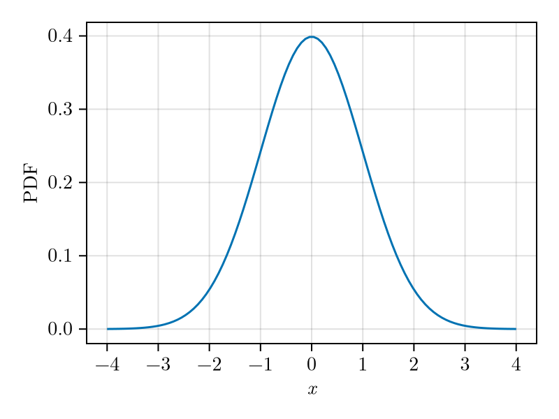
For a normal random variable \(X\) \[\begin{aligned} P(\{\abs{X - \mu_X} \ge \sigma_X\}) &\approx 0.371\\ P(\{\abs{X - \mu_X} \ge 3\sigma_X\}) &\approx 0.0027\,. \end{aligned}\]
2.2 Uniform Distribution
Let \(a,b\in\ensuremath{{\mathbb{R}}}, a < b\). A uniform distribution \(U(a,b)\) is characterised by the PDF \[\begin{equation} \label{eq:uniform-pdf} p(x) = \begin{cases} \frac{1}{b-a} & x\in (a,b)\\ 0 & \text{otherwise}\,. \end{cases} \end{equation}\] The PDF of \(U(0,1)\) is shown in Fig. 2
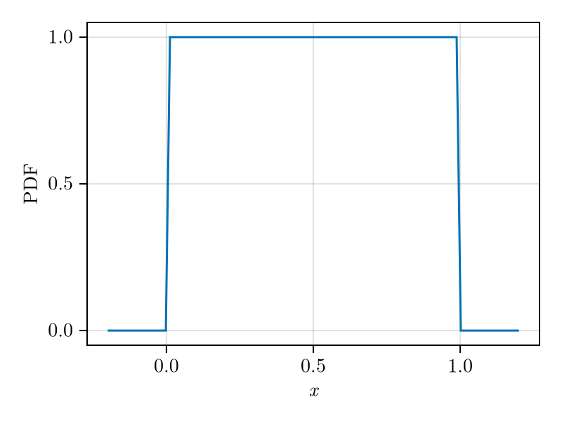
The expected value and standard deviation of a uniform random variable \(X\) are given by \[\begin{aligned} \operatorname{E}[X] &= \frac{a+b}{2}, & \sigma_X &= \frac{b-a}{\sqrt{12}}, & \mu_{X,4} &= \frac{(b - a)^4}{80}\,. \end{aligned}\] Further, for \(b - a = 1\) we have \(P(\abs{X - \mu_X} > \sqrt{3}\sigma_X) = 0\).
2.3 Independece
Two random variables \(X\) and \(Y\) are independent if for every \(-\infty \le a_i \le b_i \le \infty, i=1,2\) \[\begin{equation} \label{eq:independence-def} P_{XY}(a_1 \le X \le b_1, a_2 \le Y \le b_2) = P_X(a_1 \le X \le b_1)P_X(a_2 \le Y \le b_2)\,. \end{equation}\] In that case \[p_{XY}(x,y) = p_X(x) p_Y(y)\,.\] As a consequence \[\operatorname{E}[g(x)h(y)] = \operatorname{E}[g(x)]\,\operatorname{E}[h(y)]\] as the integrals can be separated, and \[\begin{equation} \label{eq:var-X+Y-of-indep-rv} \begin{split} \operatorname{Var}(X+Y) &= \operatorname{E}[(X + Y - \mu_X - \mu_Y)^2]\\ &= \operatorname{E}[(X - \mu_X)^2] + \operatorname{E}[(Y - \mu_Y)^2] - \operatorname{E}[(X - \mu_X)(Y - \mu_Y)]\\ & = \operatorname{Var}(X) + \operatorname{Var}(Y)\,. \end{split} \end{equation}\]
3 Sample Mean and Variance
In general one doesn’t know the distribution underlying the results of experiments affected by random processes. In that case one has to resort to statistical methods to characterise the underlying random processes.
Two fundamental statistical quantities of interest are the sample mean and variance. Let \(x_1,\dotsc,x_n\) denote the outcomes of \(n\) measurements of a random variable \(X\). The sample (aritmetic) mean is defined by \[\begin{equation} \label{eq:sample-mean-def} m = \frac{x_1 + \dotso + x_n}{n}\,, \end{equation}\] and is used to estimate the expected value of \(X\). To verify that if \(n\) is large \(m\) converges to \(\mu_X\) lets write each measurement as the sum of the true average plus an error, \(x_i = \mu_X + e_i, i=1,\dotsc,n\). We then have \[m = \frac{1}{n}\sum_{i=1}^n \mu_X + e_i = \mu_X + \frac{1}{n}\sum_{i=1}^n e_i\,.\] The second term represents the total error in the estimate of \(\mu_X\) and is a sample of a random variable. To estimate it, we assume that the errors of the individual measurements \(e_i\) are independent from each other and that they are all generated by the underlying random variable \(X\). More formally, let \(\{X_i\}_{n\ge 1}\) be a sequence of independent and identically distributed (i.i.d.) random variables equal to \(X\) such that \(\operatorname{E}[X_1^2] < \infty\). Then \[\begin{equation} \label{eq:mean-rv-def} \overline{X}_n \ensuremath{:=}\frac{X_1 + \dotso + X_n}{n} \end{equation}\] is the random variable characterising the mean and \(m = X(\omega)\) for some \(\omega\in\Omega\). The expected value of \(\overline{X}_n\) is immediately found from the linearity of the expected value operator \[\begin{equation} \label{eq:mean-rv-ev} \operatorname{E}[\overline{X}_n] = \mu_X\,. \end{equation}\] The mean error can then be estimated based on the standard deviation of \(\overline{X}_n\). Using \eqref{eq:var-X+Y-of-indep-rv} we find \[\sigma_{\overline{X}_n} = \frac{1}{n}\sqrt{\sum_{i=1}^n \sigma_X^2} = \frac{\sigma_X}{\sqrt{n}}\] which shows that the error is inversely proportional to \(\sqrt{n}\) and hence, for large \(n\), \(m\) does indeed converges to \(\mu_X\).
The (unbiased) sample variance is defined by \[\begin{equation} \label{eq:sample-var-def} s^2 = \frac{(x_1-m)^2 + \dotso + (x_n-m)^2}{n-1} \end{equation}\] and is used to estimate the true variance of the underlying random variable \(X\). To show that this is indeed the case, let \(\{X_i\}_{n\ge 1}\) and \(\overline{X}_n\) be as introduced above. Then we define the random variable \(S_n^2\) \[\begin{equation} \begin{split} S^2_n &\ensuremath{:=}\frac{1}{n-1}\sum_{i=1}^n (X_i - \overline{X})^2\\ &=\frac{1}{n-1}\sum_{i=1}^n[(X_i - \mu_X) - (\overline{X} - \mu_X)]^2\,. \end{split} \end{equation}\] and show that its expected value converges to \(\sigma_X^2\). To that end lets first use the linearity of the expected value operator and write \[\begin{split} \operatorname{E}[S^2_n] &= \frac{1}{n-1} \sum_{i=1}^n \operatorname{E}[(X_i - \mu_X)^2] + \operatorname{E}[(\overline{X}_n - \mu_X)^2]\\ &\qquad - 2\operatorname{E}[(X_i - \mu_X)(\overline{X}_n - \mu_X)]\,. \end{split}\] The first two terms of the summation are \(\sigma_X^2\) and \(\sigma_X^2/n\) respectively. To compute the expected value appearing in the last one we substitute the definition of \(\overline{X}_n\) to obtain \[\begin{split} \operatorname{E}[(X_i - \mu_X)(\overline{X}_n - \mu_X)] &= \operatorname{E}[(X_i - \mu_X) \sum_{k=1}^n \frac{X_k - \mu_X}{n}]\\ &= \frac{\operatorname{E}[(X_i - \mu_X)^2]}{n}\\ &= \frac{\sigma_X^2}{n} \end{split}\] where in the second line we used the fact that \(X_i\) and \(X_k\) for \(i\ne k\) are independent. Putting together these results we obtain \[\begin{split} \operatorname{E}[S^2_n] &= n \frac{\sigma_X^2 + \sigma_X^2/n - 2\sigma_X^2/n}{n-1}\\ &= \sigma_X^2\,. \end{split}\] The variance of \(S^2\) can be computed in a similar way and one obtains \[\operatorname{Var}(S^2) = \frac{1}{n} \Big(\mu_{X,4} - \frac{n-3}{n-1}\sigma_X^4\Big)\,,\] confirming that for \(n\) large the unbiased sample variance converges to the true variance.
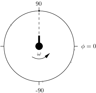
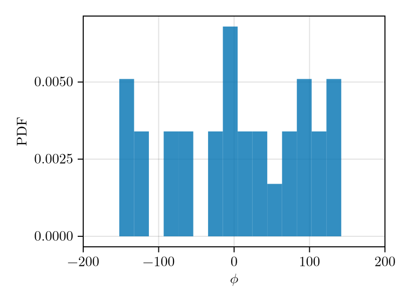
Running example part 1. A (toy) cannon rotates at a constant angular velocity \(\omega\) and fires at random times such that the probability of hitting the surrounding circle at angle \(\phi\) is uniform. The position of the hitting points is recorded by the angle \(\phi\in [-180,180)\) (see Fig. 3). The true mean and \(\sigma_X\) are \[\begin{aligned} \operatorname{E}[X] &= 0 & \sigma_X &= 103.92\,. \end{aligned}\] Using the data from one particular sample set with \(n=30\) we obtain \[\begin{aligned} m &= 6.0214 & s &\ensuremath{:=}\sqrt{s^2} = 92.123\,. \end{aligned}\] Note that in this case talking about a “\(3\sigma_X\)” margin doesn’t make sense since no sample will ever be generated at that value of \(\phi\)! The empirical PDF estimated from the samples is shown in Fig. 4. Given the small number of samples, without a-priori knowledge, it’s difficult to guess the right distribution.
4 Law of Large Numbers
In Sect. 3 we used ad-hoc considerations to show that the sample mean and variance are estimates of the expected value and variance of the underlying random variable \(X\). In this section we present a variant of the weak law of large numbers (WLLN) theorem for i.i.d. random variables which has a much broader applicability.
Theorem 1 (Weak law of large numbers). Let \(\{X_n\}_{n \ge 1}\) be a sequence of i.i.d. random variables such that \(\operatorname{E}[X_1^2]<\infty, \operatorname{E}[X_1]=\mu_X\) and \(\operatorname{Var}(X_1)=\sigma_X^2\). Then for any \(\epsilon > 0\) \[\begin{equation} \label{eq:weakk-law-of-large-num} \lim_{n\to\infty} P(\abs{\overline{X}_n - \mu_X} > \epsilon) = 0\,. \end{equation}\] One says that \(\overline{X}_n\) converges in probability to \(\operatorname{E}[X_1]\).
Proof. Let \(Y\) be a random variable with \(\operatorname{E}[Y^2]<\infty\) and \(a>0\), then \[\begin{split} \sigma_Y^2 &= \int_{-\infty}^\infty x^2 p_Y(x) \mathrm{d}x \ge \int_{\abs{x}\ge a\sigma_Y} x^2 p_Y(x) \mathrm{d}x\\ &\ge a^2\sigma_Y^2 \int_{\abs{x}\ge a\sigma_Y} p_Y(x) \mathrm{d}x = a^2\sigma_Y^2 P(\abs{Y} \ge a\sigma_Y)\,. \end{split}\] Setting \(Y=X_1 - \mu_X\) and rearranging we obtain Chebyshev’s inequality \[\begin{equation} \label{eq:chebyshevs-ineq} P(\abs{X_1 - \mu_X} \ge a\sigma_X) \le \frac{1}{a^2}\,. \end{equation}\] Finally, applying this inequality to the probability of the theorem with \(a\sigma_X = \epsilon\) we obtain \[P(\abs{\overline{X}_n - \mu_X} > \epsilon) \le \frac{\sigma_X^2}{n\epsilon^2}\] which shows that \(\lim_{n\to\infty} \frac{\sigma_X^2}{n\epsilon^2} = 0\). ◻
Note that \(S^2\) is a random variable. If the conditions of the weak law of large numbers are satisfied, it converges in probability to \(\sigma_X^2\) which implies that its standard deviation converges to 0.
5 Central Limit Theorem
Up to this point we developed methods to estimate the mean and the variance of random variables from samples. However, without knowledge about the distribution of the mean, the standard deviation only gives qualitative indication of the uncertainty of the estimate. The central limit theorem (CLT) is a fundamental tool enabling quantitative assertions about the latter.
Theorem 2 (Central limit theorem for i.i.d. random variables). Let \(\{X_n\}_{n \ge 1}\) be a sequence of i.i.d. random variables such that \(\operatorname{E}[X_1]=\mu_X\) and \(\operatorname{Var}(X_1)=\sigma_X^2 < \infty\). Further, let \(F_\mathcal{N}\) be the CDF of \(\mathcal{N}(0,\sigma_X^2)\) and \(F_n\) the one of \[Y_n = \sqrt{n}(\overline{X}_n - \mu_X)\] with \[\overline{X}_n \ensuremath{:=}\frac{X_1 + \dotso + X_n}{n}\,.\] Then \[\lim_{n\to\infty} F_n(x) = F_\mathcal{N}(x), \qquad x\in\ensuremath{{\mathbb{R}}}\,.\] One says that \(Y_n\) converges in distribution to \(\mathcal{N}(0,\sigma_X^2)\).
The theorem shows that, for \(n\) large, the distribution of the random variable \(\overline{X}_n\) converges to a normal distribution with expected value \(\mu_X\) and variance \(\sigma_X^2/n\). Note that \(X_1\) doesn’t need to be Gaussian. A proof and generalisations can be found in [1].
For sufficiently large \(n\) one can therefore estimate the uncertainty of means based on the normal distribution of the limit rather than on the much more difficult to evaluate \(F_n\).
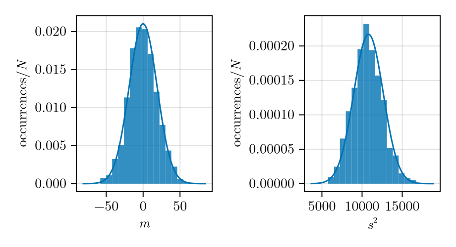
Running example part 2. To verify in our running example how close \(\overline{X}_n\) and \(S^2_n\) are to a normal distribution when \(n=30\), we run 1000 times the experiment. The resulting empirical PDFs are shown in Fig. 5 together with the limiting distributions (\(n\to\infty\)) according to the CLT. The mean looks fairly close to the limiting normal distribution. From the CLT the standard deviation of the 30 sample mean converges to \[\sigma_{\overline{X}} = \frac{\sigma_X}{\sqrt{n}} = 18.97\,.\] The unbiased sample standard deviation computed from the means \(m_1,\dotsc,\allowbreak m_{1000}\) of the 1000 runs is 19.21 in reasonable agreement.
Similarly, the CLT says that \(s\) converges to \[\sqrt{\mu_{S^2}} = \sigma_X = \frac{360}{\sqrt{12}} = 103.92\] and the mean of the 1000 runs \(s_1,\dots,s_{1000}\) gives 102.91, also in fairly good agreement. Note however that the empirical PDF of \(s^2\) is slightly asymmetric. To obtain a PDF closer to a Gaussian distribution, \(n\) has to be increased.
6 Confidence Intervals
Sample means are random variables. It is therefore important to specify the uncertainty in the calculated value. The confidence interval is a common way to indicate it.
Given a data set and a mean \(m\) calculated from it, the confidence interval (CI) specifies an interval \((u(\overline{X}_n), v(\overline{X}_n))\) within which the real value of the mean \(\operatorname{E}[\overline{X}_n]\) is believed to lie with confidence level \(p\) (95% and 99% are typical values for \(p\)) \[P(u(\overline{X}_n) < \operatorname{E}[\overline{X}_n] \le v(\overline{X}_n)) = p\,.\] The interval limits are themselves random variables. The confidence level (or coefficient) indicates that, if we would computed the interval a large number of times (on different data sets), then a fraction \(p\) of them would contain the true value \(\operatorname{E}[\overline{X}_n]\).
6.1 Known Variance Case
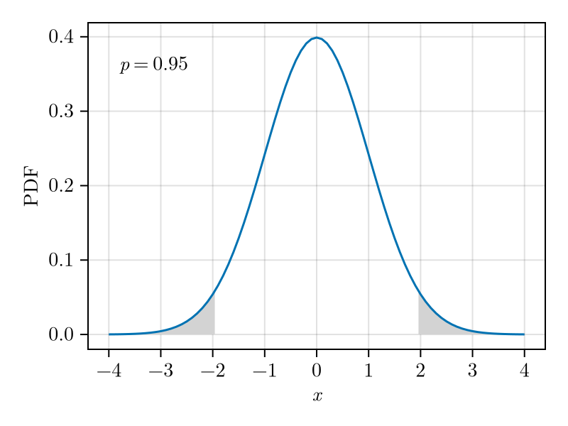
Let \(X\) be a random variable of unknown distribution but known variance \(\sigma_X^2\). Then the central limit theorem tell us that, for \(n\) large, the distribution of \(\overline{X}_n\) converges to a normal distribution with variance \(\sigma_X^2/n\). The CLT therefore enable us to calculate a confidence interval.
Let \(m\) denote the sample mean calculated from a data set, \(F_\mathcal{N}\) the CDF of \(\mathcal{N}(0, 1)\) and \(p\) the confidence interval. Then \[\begin{split} p &= \int_{-C}^C p_\mathcal{N}(x) \mathrm{d}x = F_\mathcal{N}(C) - F_\mathcal{N}(-C)\\ &= F_\mathcal{N}(C) - (1 - F_\mathcal{N}(C)) = -1 + 2F_\mathcal{N}(C)\,, \end{split}\] from which we can compute \(C\) \[C = F_\mathcal{N}^{-1}\Bigl(\frac{1 + p}{2}\Bigr)\,.\] The symmetric \(p\)-confidence interval is therefore \[m - C\frac{\sigma_X}{\sqrt{n}} < \mu_X < m + C \frac{\sigma_X}{\sqrt{n}}\,.\]
Running example part 3. In our running example the standard deviation is known. We can therefore compute a confidence interval as outlined in this section. From \(p=0.95\) we obtain \(C\approx 1.96\). Hence the confidence interval calculated from the first run (\(m_1\)) is \[-31.16 \le \mu_X \le 43.20\,.\] In this case the interval includes the real \(\mu_X\) value. However, due to the small sample number, the interval is fairly large.
6.2 Unknown Variance Case
In many situations the variance of the random variable underlying an experiment is not known. In this case, if the underlying distribution is known to be normal, one can use Student’s t distribution to estimate the uncertainty in the calculated mean \(m\) even for small values of \(n\ge 2\).
Let \(\{X_1,\dotsc,X_n\}_{n\ge 1}\) be i.i.d. normal random variables with expected value \(\mu_X\) and variance \(\sigma_X^2\). The sum of normal random variables is also normal. Therefore, from the CLT, \(\overline{X}_n\) is a Gaussian random variable with variance \(\sigma_X^2/n\) and \[Z = (\overline{X}_n - \mu_X)\frac{\sqrt{n}}{\sigma_X}\] a 0 centred Gaussian random variable of variance 1 (\(\mathcal{N}(0,1)\)).
For normal random variables \(X_i, i=1,\dotsc,n\) it can be shown that the unbiased sample mean \(S^2_n\) is a scaled \(\chi^2\) random variable and that it is independent of \(Z\) [2]. Let \(V_\nu\) be a \(\chi^2\) distributed random variable with \(\nu=n-1\) degrees of freedom. It’s relationship to \(S^2_n\) is \[V_\nu = \nu\frac{S^2_{\nu+1}}{\sigma_X^2}\,.\] Then the ratio \[T = \frac{Z}{\sqrt{V_{n-1}/(n-1)}} = (\overline{X}_n - \mu_X)\frac{\sqrt{n}}{S_n}\] is a symmetric, 0 centred random variable that doesn’t depend on \(\sigma_X\). It’s PDF is given by [3] \[p_T(t;\nu) = \frac{\Gamma\big(\frac{\nu+1}{2}\big)} {\sqrt{\pi \nu}\Gamma\bigl(\frac{\nu}{2}\bigr)} \frac{1}{\big(1 + \frac{t^2}{\nu}\big)^{(\nu+1)/2}}\] with \(\Gamma\) the Gamma function. It is called the Student \(t\) distribution and is shown in Fig. 7 for various values of \(\nu=n-1\). For comparison the figure also shows the PDF of an \(\mathcal{N}(0,1)\) random variable and makes it apparent that for small values of \(n\) the Student \(t\) PDF has a longer tail than \(\mathcal{N}(0,1)\). As \(n\) increases the difference reduces and for \(n \gtrapprox 30\) the Student \(t\) distribution becomes very similar to the standard normal one.
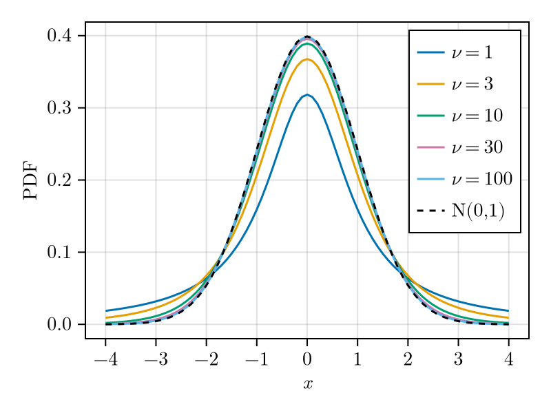
A \(p\)-confidence interval for the mean can be calculated as in Sect. 6.1 by replacing \(F_\mathcal{N}\) by \(F_T\), the CDF of \(T\), and using \(s\) instead of the unknown \(\sigma_X\) \[m - C\frac{s}{\sqrt{n}} < \mu_X < m + C \frac{s}{\sqrt{n}}\,.\]
If the random variable \(X_1\) is not normally distributed, then one can only use the Student \(t\) distribution to estimate confidence intervals for large degrees of freedom \(\nu=n-1\). In fact, under the assumption of large \(n\), the CLT teaches us that all means of random variables with finite variance converge to a Gaussian distribution. What the Student \(t\) distribution adds, is that the error introduced by using the unbiased sample variance estimate \(s^2_n=S^2_n(\omega)\) instead of the unknown \(\sigma_X^2\) becomes negligible. How large \(n\) needs to be for an estimate to a desired accuracy depends on the distribution of \(X_1\).
Running example part 4. If in our running example we didn’t know the standard deviation, we could use the Student \(t\) distribution to estimate a confidence interval. In this case, for \(p=0.95\) and \(\nu=n-1=29\), the value of \(C\) would be slightly larger at 2.04 and, from the data of the first run \(m_1\) and \(s_1\) we’d obtain the interval \[-28.29 \le \mu_X \le 40.33\,.\]
6.3 Summary
In this document we introduced the sample mean and unbiased sample variance and showed that they are estimates for the expected value and variance of the random variable underlying the experiment. We also computed the variance of both of them and showed that as the number of samples increases (\(n\to\infty\)), they converge to 0 as \(\propto 1/n\). In other words, the sample mean and unbiased sample variance converge to the true values of the measured quantity. This fact is generalised to any mean by the weak law of large numbers which we stated and proved. These results are important, but if the underlying distribution is unknown, they only permit qualitative descriptions.
We then introduced the central limit theorem which shows that, under mild conditions, every mean converges to a normal distribution. With this tool in the hands we can make quantitative assertions. In particular we introduced the concept of confidence interval which is an indication of where the true value of the quantity of interest is believed to lie with a specified confidence level \(p\).
References
\(\ensuremath{{\mathcal{P}}}(\Omega)\) is the power set of \(\Omega\), i.e., the set of all subsets of \(\Omega\).↩︎
